Scikit-learn is one of the most fundamental machine learning tools. You could access its official website here. It may not as fancy as pytorch or tensorflow, but scikit-learn is a good starting point for beginners to learn about machine learning algorithms. In this tutorial, several aspects will be shown, including installation, datasets as well as applying several machine learning algorithms to the introduced data sources.
The source code files in this tutorial
are accessible from Canvas1, in addition, you could also access the resources from Google Colab, please make sure that you are using your VT’s Google Account to access the code, it will direct you to the google drive interface, you only have to click open with google colaboratory to open up the code using google colab. For Google Colab it is easier for you to run python code as you don’t have to manually install the machine learning packages.
Update History
2024 November 22: Fix the images issue, fix original url compatibility issue, add acknowledgement section.
2023 November 26: Explanation contents suggested by Prof. Sarkar.

Calendar ICS file: here.
2023 November 11: Initial update.
Interacting with Notebooks
For machine learning based demonstrations, the programming language python is widely used because it is free, portability and module design. In addition to running machine learning based algorithms on python scripts like we normally do, a new type of file is used named Jupyter notebooks with the extension of ipynb. The main different between a Jupyter notebook and a python script is that Jupyter notebook is more versatile and much easier to use than a Pyhon script. Jupyter notebook can run part of the coding blocks where as for a python script, it needs to be executed from beginning to end, the problem is that the training phase of many machine learning algorithms are time consuming, sometimes one may not want to retrain the model but wish to do some evaluations work still has to run the whole script to see the results. Jupyter notebook is more useful in terms of machine learning applications.
In order to run the Jupyter notebooks, you can run it on you computer with visual studio code, but there are online services like Google Colab that allows its users to run Jupyter notebooks with breeze. You can decide which way you want to run. For the rest of the tutorial, Jupyter notebook will be used for demonstration.
library Installation
This part is going to introduce you some of the most commonly used machine learning libraries that could be helpful for your projects. These are beginner friendly yet are powerful to use. If you want to check out the details of each of the library you could visit the official website for each of the packages and gain better understandings of the details under the hood. This part is mainly used for users who are trying to run their notebooks on their local machine.
scikit-learn library
To install it on your local machine or server, run the following commands depending on your OS, you could also check out the official installation guide:
Even through there are 2 types of commands to install the modules on python, they both use the pip module that is built-in to the python package. For the 2nd type of command: python will use the module by using -m pip to invoke the module to install packages.
For windows:
pip install -U scikit-learn;
python -m pip install -U scikit-learn;
For macOS and Linux:
pip3 install -U scikit-learn;
python3 -m pip install -U scikit-learn;
You can verify the installations by running the following commands:
python -m pip show scikit-learn  # to see which version and where scikit-learn is installed
python -m pip freeze  # to see all packages installed in the active virtualenv
python -c "import sklearn; sklearn.show_versions()"
Based on the previous examples on how to install packages, you could also install pandas and other tools on your local machine.
Additional libraries for Machine Learning
Additional libraries will be liested here that will be used for the tutorial as well as for your project. They could be installed the way scikit-learn is installed shown above.
matplotlib
Matplotlib is a comprehensive library for creating static, interactive, and animated visualizations in Python. Conceived by John Hunter in 2003 to emulate the plotting capabilities of MATLAB within Python, it has since become the de facto standard plotting library within the Python data science ecosystem. Matplotlib provides a vast array of functions and tools to generate plots, histograms, power spectra, bar charts, error charts, scatterplots, etc., with just a few lines of code. Its design is highly customizable and extendable, allowing for the creation of complex plots suited for a wide range of contexts. The library integrates well with many data manipulation tools in Python, such as NumPy and pandas, and it is supported by many environments that enable Python plotting, such as Jupyter notebooks. Its versatility makes it an invaluable tool for exploratory data analysis, scientific computing, and the production of publication-quality figures.
pandas
Pandas is an open-source data analysis and manipulation tool in Python, pivotal for modern data science tasks. It provides fast, flexible, and expressive data structures designed to work with both “relational” or “labeled” data effortlessly. The core of pandas is its DataFrame, a powerful two-dimensional tabular structure with labeled axes (rows and columns) that can hold heterogeneous data types. Developed by Wes McKinney, pandas simplifies the process of data cleaning, transformation, and analysis. It integrates well with other data science and machine learning libraries, supporting a wide range of file formats and databases. With its comprehensive feature set for operations such as slicing, filtering, merging, and reshaping datasets, pandas is an indispensable toolkit for any data-intensive Python application.
misc
The essential libraries are provided above as you already know how to use the Python package manager to install libraries. In the future, you may need to learn about anaconda, venv, as well as other libraries like Pytorch and Tensorflow, which are much more complex. These are out of the topic for this post, but you could explore in the future.
Datasets in scikit-learn
Datasets play a pivotal role in machine learning, serving as the foundation upon which models are trained, tested, and validated. High-quality datasets are essential for creating accurate and robust machine learning models, as they provide the necessary information for algorithms to learn patterns, make predictions, and generalize to new, unseen data. In scikit-learn, several widely used datasets are readily available. These include the Iris dataset, which is used for classification tasks, the Boston Housing dataset for regression, and the Breast Cancer Wisconsin (Diagnostic) dataset for binary classification. These datasets, among others, serve as excellent starting points for exploring machine learning techniques and developing models for various tasks, making scikit-learn a valuable resource for both beginners and experienced practitioners in the field.
This table is going to list some of the most widely used datasets across the machine learning research area, the links to scikit-learn are provided, you could check them out by clicking on the embedded hyperblink at the name in the first column.
| Name | Type | Brief Introduction |
|---|---|---|
| Iris | Classification | A classic dataset for multi-class classification. It consists of three species of iris flowers, with four features each. |
| Wine | Classification | A dataset for wine classification with 13 features. |
| Breast Cancer | Classification | Used for binary classification, containing breast cancer data. |
| Diabetes | Regression | A dataset for regression tasks, focusing on diabetes. |
| Linnerud | Multivariate Regression | Includes physiological and exercise data for multiple regression. |
| Olivetti Faces | Classification | Consists of grayscale images of 40 people’s faces. |
| 20 Newsgroups | Text Classification | A collection of newsgroup documents for text classification. |
| Digits | Classification | Handwritten digits dataset for digit recognition. |
| Labeled Faces in the Wild (LFW) | Face Recognition | A face recognition dataset containing images of celebrities. |
| Olivetti Faces | Classification | A dataset of facial images for classification tasks. |
| California Housing | Regression | Housing price prediction dataset for regression. |
| Randomized Isolated Forest (RIF) | Anomaly Detection | A synthetic dataset for anomaly detection. |
Iris dataset
In this tutorial Iris dataset2 is mainly used as it is easy for beginners to understand and intepret. The Iris dataset is a foundational dataset for statistics and machine learning, often used for teaching purposes in the areas of classification and data analysis. Comprising 150 samples collected from three species of Iris flowers—Setosa, Versicolour, and Virginica—the dataset contains four features for each sample: the length and the width of the sepals and petals in centimeters. Originally collected by biologist and statistician Ronald Fisher in the 1930s, the dataset has become a case study in multivariate data analysis. Its simplicity and small size allow for clear visualization and understanding of the data, making it ideal for demonstrating the principles of machine learning algorithms, especially in categorizing objects into predefined classes. Its use has been so widespread in the field of machine learning that it’s often referred to as the “hello world” of datasets.
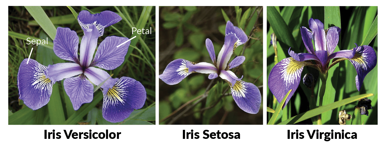
Sepals and petals are two types of organ that constitute the parts of a flower, and they are both crucial features in the Iris dataset. In botany, sepals are typically the outermost part of a flower, looking similar to leaves, that protect the developing bud. Petals are the often colorful segments that follow the sepals, which serve to attract pollinators such as insects and birds with their vivid colors and unique patterns. In the Iris dataset, the length and width of these sepals and petals are measured and recorded for each iris flower specimen. These measurements form the basis of the dataset’s features, providing data points that are used to distinguish between the three different Iris species included in the study. By analyzing variations in sepal and petal dimensions, machine learning models can be trained to identify and predict the species of iris flowers with high accuracy, making these features fundamental to the dataset’s utility in classification tasks. Referring from the article, the following 2 images how the projection looks like from features to data.
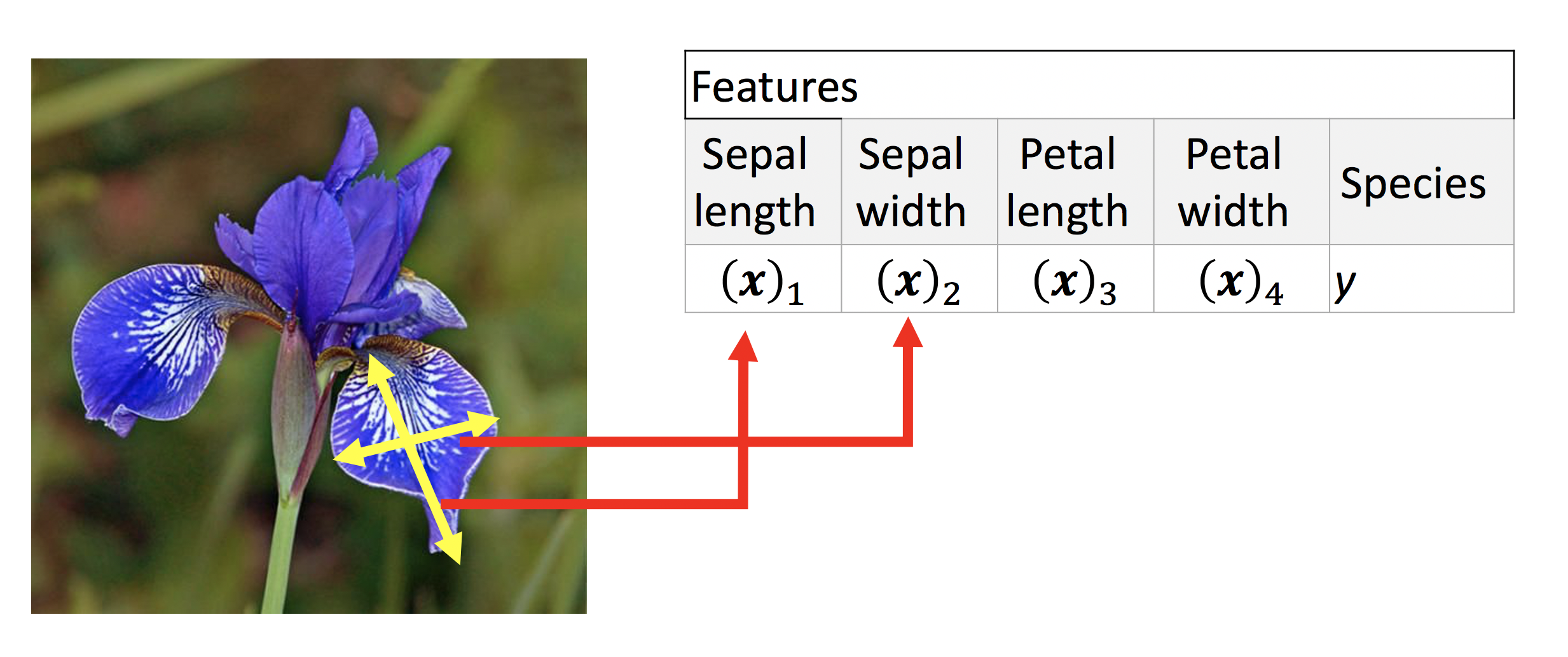
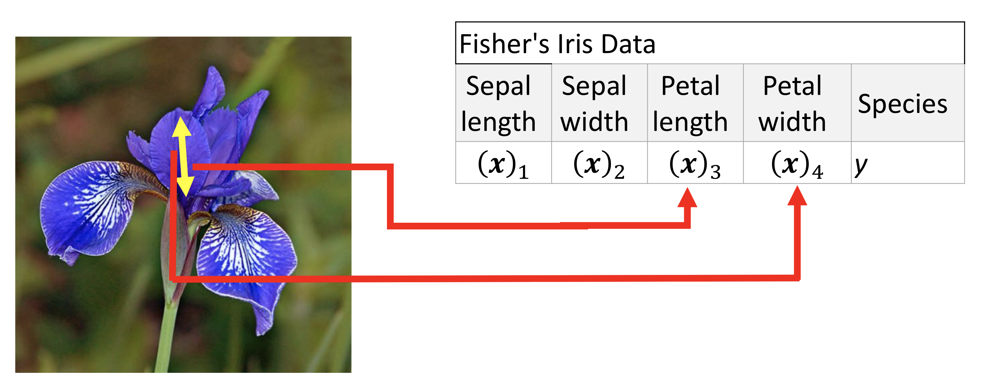
The following code snippet provides a parallel coordinate plot of the Iris dataset.
import seaborn as sns
import matplotlib.pyplot as plt
from pandas.plotting import parallel_coordinates
import pandas as pd
# Parallel Coordinates
# Load the data set
iris = sns.load_dataset("iris")
parallel_coordinates(iris, 'species', color=('#556270', '#4ECDC4', '#C7F464'))
plt.legend(loc='best', fancybox=True, shadow=True)
plt.title('Parallel Coordinates Plot of Iris Data', fontsize=20, fontweight='bold', y=1.05,)
plt.show()The dataset could be shown as follows if we use either sepal features or petal features.
For the sepal features, according to the following code, the graph would be generated regarding the various calsses for the dataset.
from sklearn import datasets
import matplotlib.pyplot as plt
iris = datasets.load_iris()
_, ax = plt.subplots()

scatter = ax.scatter(iris.data[:, 0], iris.data[:, 1], c=iris.target)
ax.set(xlabel=iris.feature_names[0], ylabel=iris.feature_names[1])
_ = ax.legend(
    scatter.legend_elements()[0], iris.target_names, loc="lower right", title="Classes"
)
plt.title("Iris dataset with sepal length and width")
ax.grid(which='both', linestyle='dotted', linewidth=0.3)
plt.show()Similarly, the petal feature based graph could be generated as follows:
from sklearn import datasets
import matplotlib.pyplot as plt
iris = datasets.load_iris()
_, ax = plt.subplots()

scatter = ax.scatter(iris.data[:, 2], iris.data[:, 3], c=iris.target)
ax.set(xlabel=iris.feature_names[2], ylabel=iris.feature_names[3])
_ = ax.legend(
    scatter.legend_elements()[0], iris.target_names, loc="lower right", title="Classes"
)
plt.title("Iris dataset with petal length and width")
ax.grid(which='both', linestyle='dotted', linewidth=0.3)
plt.show()We can produce a pair plot for the Iris dataset using the seaborn library. In the pair plot, the diagonal shows the distribution of the data for each feature. The scatter-plots for each combination of features are shown in the upper and lower triangles of the figure.
import seaborn as sns
from seaborn import pairplot
iris = sns.load_dataset("iris")
# Pair Plot
pairplot(iris, hue='species')
plt.legend(loc='best')
plt.show()You could easily see the dataset by running the following code snippet in the Jupyter notebook.
#this code block only works in Jupyter notebook
from sklearn import datasets
iris = datasets.load_iris()
iris.data
Performance measurement
Before diving into the details on various machine learning algorithms it is essential to have some knowledge on how to measure the performance of elementary machine learning models performance measurement. For classification based machine learning models, accuracy is one of the most widely used metric as it is trying to find out how the classification results compared with the actual results.
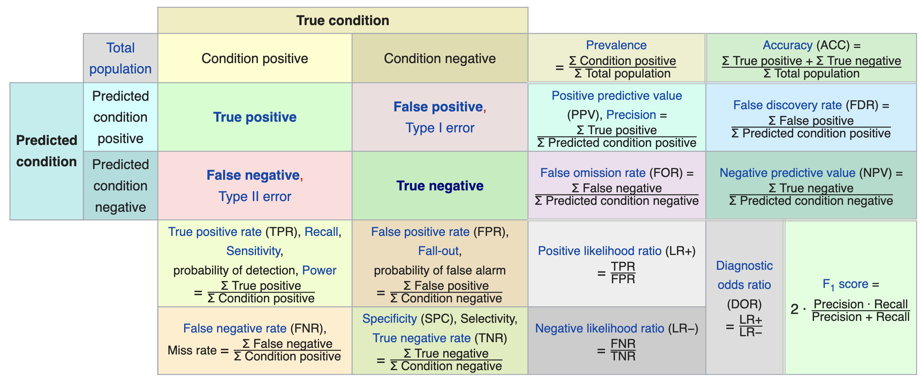
Another useful metric is called “confusion matrix”. A confusion matrix is a fundamental tool in machine learning and statistics used to evaluate the performance of a classification model. It provides a clear and concise summary of the model’s predictions by comparing them to the actual class labels in a dataset. The matrix is typically organized into four quadrants: true positives (TP), true negatives (TN), false positives (FP), and false negatives (FN). TP represents the number of correctly predicted positive instances, TN represents the number of correctly predicted negative instances, FP represents the number of false positive predictions, and FN represents the number of false negative predictions. By analyzing the values in these quadrants, one can calculate various performance metrics such as accuracy, precision, recall, and F1-score, which are essential for assessing the model’s effectiveness in solving classification problems. Confusion matrices are invaluable tools for understanding the strengths and weaknesses of a machine learning model, making them a critical component of model evaluation and optimization. Here is an image of how confusion matrix looks like3.
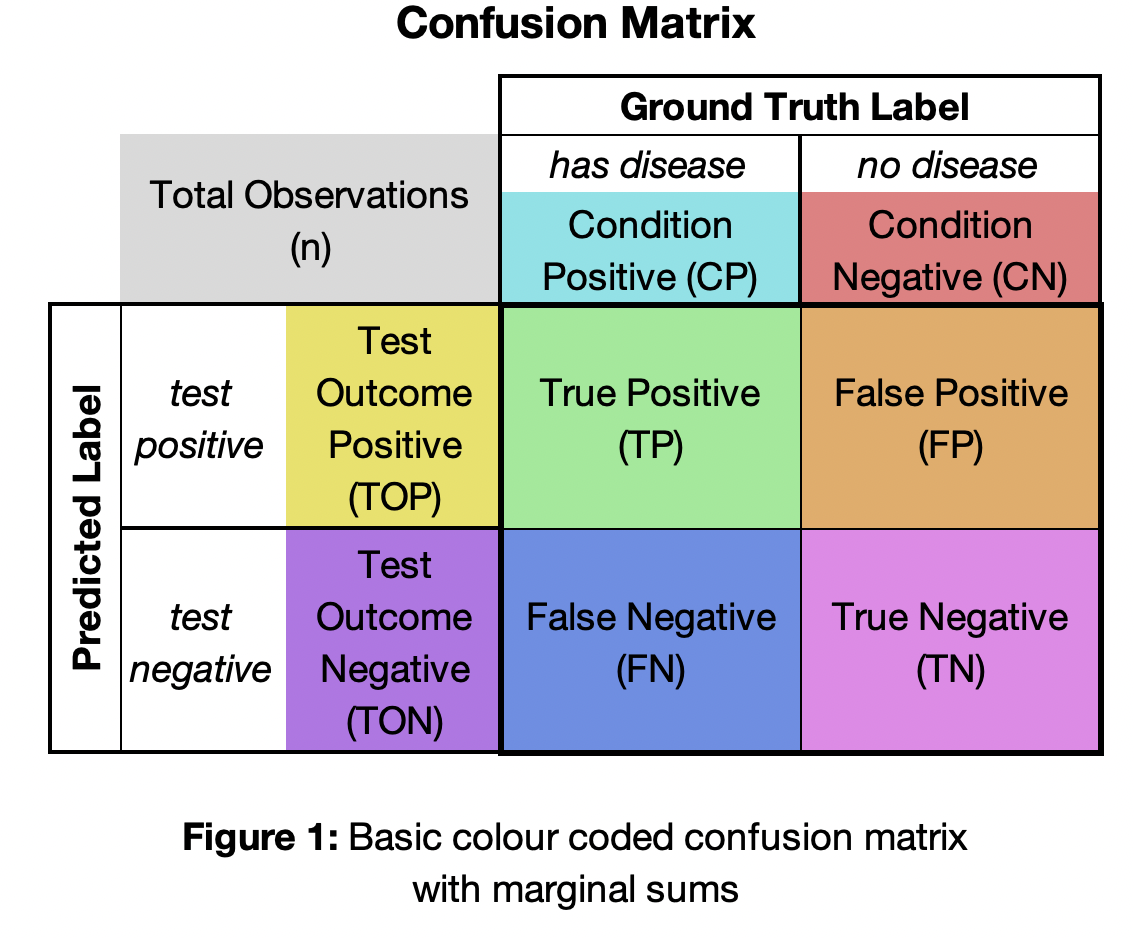
Here’s another great illustration4 about the confusion matrix that contains parameters like recall, fall-out, prevalence, accuracy, precision as well as F1 score. All those parameters are derived from the confusion matrix.
ML algorithms using scikit-learn
In the beginning of ths section, I’d like to give you a bird’s eye view of the machine learning domain. Mainly there 3 kinds of machine learing techniques, supervised learning, unsupervised learning as well as reinforcement learning. Since you have learned reinforcement learning, more will be stressed on supervised learning and unsupervised learning, in this tutorial, we are trying to use supervised learning techniques to achieve various goals like clasification. Here are some useful links that you could explore in scikit-learn.
In this article, I’m going to focus on the following machine learning algorithms based on the Iris Dataset prestend above:
The dataset in the post for demonstration is named iris which is included in scikit-learn package.
This tutorial only emphasize on the application side of the machine learning algorithms, which means the implementation of the python code. You could refer to the lecture notes as well as other resources on the internet to have better understandings of the theoretical aspects of the machine learning algorithms.
Naïve Bayes
Naïve Bayes method uses Bayes’ thorem with the assumption of conditional independence between every pair of features given class value variable.
The following equation illustrates the Bayes’ theorem of class variable \(y\) with feature vector from \(x_{1}\cdots x_{n}\).
P\left(y \mid x_{1}, \ldots, x_{n}\right)=\frac{P(y) P\left(x_{1}, \ldots, x_{n} \mid y\right)}{P\left(x_{1}, \ldots, x_{n}\right)}Using the naive conditional independence assumption:
P\left(x_{i} \mid y, x_{1}, \ldots, x_{i-1}, x_{i +1}, \ldots, x_{n}\right)=P\left(x_{i} \mid y\right)The conditional probability of \(y\) could be modified to:
P\left(y \mid x_{1}, \ldots, x_{n}\right)=\frac{P(y) \prod_{i-1}^{n} P\left(x_{i} \mid y\right)}{P\left(x_{1}, \ldots, x_{n}\right)}Thus the final steps shows the relatioinship between the conditional probability of \(y\) and the nominator, as the denominator is constant.
P\left(y \mid x_{1}, \ldots, x_{n}\right) \propto P(y) \prod_{i=1}^{n} P\left(x_{i} \mid y\right)The prediction of class value \(y\) could be acquired as follows:
\hat{y}=\arg \max _{y} P(y) \prod_{i=1}^{n} P\left(x_{i} \mid y\right)The following code snippet is used to illustrate the Naïve Bayes model, this is a general approach for most of the supervised machine learning workflow, that contains the following parts:
- import essential libraries.
- data splitting
- model initialization
- model training
- model prediction
- model evaluatoin
import pandas as pd
from sklearn.model_selection import train_test_split
from sklearn import datasets
from sklearn.naive_bayes import GaussianNB

# Load dataset
iris = datasets.load_iris()
X_train, X_test, y_train, y_test = train_test_split(iris.data, iris.target, test_size=0.2, random_state=42)

# Create and fit model
nb_model = GaussianNB()
nb_model.fit(X_train, y_train)

# Predict and evaluate
nb_predictions = nb_model.predict(X_test)
print(f"Naive Bayes Accuracy: {nb_model.score(X_test, y_test)}")
The dataset needs to be splitted apart to training and testing datasets to avoid overfitting, meaning the model is less general than what we want it to be trained, the data splitting is done as follows:
X_train, X_test, y_train, y_test = train_test_split(iris.data, iris.target, test_size=0.2, random_state=42)The parameter random_state is used to generate a randomized data splitting results, it can be any integer value that you put into.
The perforamance is described using the following lines of code:
# Predict and evaluate
nb_predictions = nb_model.predict(X_test)
print(f"Naive Bayes Accuracy: {nb_model.score(X_test, y_test)}")
It would indicate how well the trained Naïve Bayes model performs with the testing data, in this case, the output is shown as follows:
Naive Bayes Accuracy: 1.0In addition to the above code demo, you could have a look at this tutorial for this model using scikit-learn, it contains the information on theoretical aspect for Naive Bayes model. In addition, it also illustrates the usage of the model using scikit-learn python code.
As we consider naive bayses model each feature is independent of each other, the likelihood of the data is the product of the likelihood of each feature. We choose the normal distribution as the likelihood of each feature.
\begin{aligned}
P\left(X_{i} \mid Y=y_{k}\right) & =N\left(X_{i} \mid \mu_{i k}, \sigma_{i k}\right) =\frac{1}{\sqrt{2 \pi \sigma_{i k}^{2}}}e^{ \left\{-\frac{1}{2}\left(\frac{x-\mu_{i k}}{\sigma_{i k}}\right)^{2}\right\}}
\end{aligned}
\hat{\mu}_{i k}=\frac{\sum_{n} X_{i}^{(n)} \delta\left(Y^{(n)}=y_{k}\right)}{\sum_{n} \delta\left(Y^{(n)}=y_{k}\right)}\hat{\sigma}_{i k}^{2}=\frac{\sum_{n}\left(X_{i}^{(n)}-\hat{\mu}_{i k}\right)^{2} \delta\left(Y^{(n)}=y_{k}\right)}{\sum_{n} \delta\left(Y^{(n)}=y_{k}\right)}The following code will generate the figure of class-conditional density contours. The code contains tensorflow package which is out of the scope of this course. You can just run the code and see the figure. The thought and code are referred from article “Probabilistic Deep Learning with Tensorflow”5.
import tensorflow as tf
import tensorflow_probability as tfp
tfd = tfp.distributions
import numpy as np
import matplotlib.pyplot as plt
from sklearn.metrics import accuracy_score
from sklearn import datasets, model_selection
from google.colab import files

%matplotlib inline

iris = datasets.load_iris()
# Use only the first two features: sepal length and width

data = iris.data[:, :2]
targets = iris.target

x_train, x_test, y_train, y_test = model_selection.train_test_split(data, targets, test_size=0.2)

labels = {0: 'Iris-Setosa', 1: 'Iris-Versicolour', 2: 'Iris-Virginica'}
label_colours = ['blue', 'orange', 'green']

def get_meshgrid(x0_range, x1_range, num_points=100):
    x0 = np.linspace(x0_range[0], x0_range[1], num_points)
    x1 = np.linspace(x1_range[0], x1_range[1], num_points)
    return np.meshgrid(x0, x1)


def plot_data(x, y, labels, colours):
    for c in np.unique(y):
        inx = np.where(y == c)
        plt.scatter(x[inx, 0], x[inx, 1], label=labels[c], c=colours[c])
    plt.title("Training set")
    plt.xlabel("Sepal length (cm)")
    plt.ylabel("Sepal width (cm)")
    plt.legend()

def get_class_conditionals(x, y):
    mu = [np.mean(x[y == k], axis=0) for k in range(3)]
    sigma = [np.sqrt(np.mean( (x[y == k]-mu[k])**2, axis=0) ) for k in range(3)]
    return tfd.MultivariateNormalDiag(loc=mu, scale_diag=sigma)

def contour_plot(x0_range, x1_range, prob_fn, batch_shape, colours, levels=None, num_points=100):
    X0, X1 = get_meshgrid(x0_range, x1_range, num_points=num_points)
    Z = prob_fn(np.expand_dims(np.array([X0.ravel(), X1.ravel()]).T, 1))
    #print(Z.shape, batch_shape, 'x', *X0.shape)
    Z = np.array(Z).T.reshape(batch_shape, *X0.shape)
    for batch in np.arange(batch_shape):
        if levels:
            plt.contourf(X0, X1, Z[batch], alpha=0.2, colors=colours, levels=levels)
        else:
            plt.contour(X0, X1, Z[batch], colors=colours[batch], alpha=0.3)


plt.figure(figsize=(10, 6))
plot_data(x_train, y_train, labels, label_colours)
x0_min, x0_max = x_train[:, 0].min(), x_train[:, 0].max()
x1_min, x1_max = x_train[:, 1].min(), x_train[:, 1].max()

class_conditionals = get_class_conditionals(x_train, y_train)
contour_plot( (x0_min, x0_max), (x1_min, x1_max), class_conditionals.prob, 3, label_colours)
plt.title("Training set with class-conditional density contours")
plt.grid("minor", linestyle='--')Linear Regression
This article contains the equation of linear regression, simply put, it tries to model the relationship between predictors and labels in a linear relationship. Based on wikipedia, linear regression could be described in the following equation:
\left[\begin{array}{c}
y_{1} \\
y_{2} \\
\vdots \\
y_{n}
\end{array}\right]=\left[\begin{array}{cccc}
1 & x_{11} & \cdots & x_{1 p} \\
1 & x_{21} & \cdots & x_{2 p} \\
\vdots & \vdots & \ddots & \vdots \\
1 & x_{n 1} & \cdots & x_{n p}
\end{array}\right]\cdot \left[\begin{array}{c}
\beta_{0} \\
\beta_{1} \\
\beta_{2} \\
\vdots \\
\beta_{p}
\end{array}\right]+\left[\begin{array}{c}
\varepsilon_{1} \\
\varepsilon_{2} \\
\vdots \\
\varepsilon_{n}
\end{array}\right]
The matrix \(\mathbf{y}\) is the observed value, where matrix \(\mathbf{X}\) is the regressors, \(\mathbf{\beta}\) is the regression coefficients, the last term \(\mathbf{\varepsilon}\) is named error term or noise. Linear regression assumes that relationship between observed value and regressors has a linear relationship.
The following code snippets illustrates how the linear regression model can be used on Iris dataset, the basic workflow is similar to the previous Naïve Bayes model. As one could tell, this is a regression model rather than the role of classification, this code snippet to find the linear relationship between sepal length and petal length.
# Step 1: Import required libraries
from sklearn import datasets
from sklearn.model_selection import train_test_split
from sklearn.linear_model import LinearRegression
import matplotlib.pyplot as plt

# Step 2: Load the Iris dataset
iris = datasets.load_iris()
X = iris.data[:, :1]  # we're using only one feature for simplicity, sepal length
y = iris.data[:, 2]   # target will be petal length, normally this would be a class

# Step 3: Split the dataset into training and test sets
X_train, X_test, y_train, y_test = train_test_split(X, y, test_size=0.2, random_state=0)

# Step 4: Create a linear regression model
model = LinearRegression()

# Step 5: Train the model using the training sets
model.fit(X_train, y_train)

# Step 6: Make predictions using the test set
y_pred = model.predict(X_test)

# Step 7: Plot outputs
plt.scatter(X_test, y_test, color='darkslategray', label='Actual')
plt.plot(X_test, y_pred, color='indigo', linewidth=3, label='Predicted')
plt.xlabel('Sepal Length (cm)')
plt.ylabel('Petal Length (cm)')
plt.title('Linear Regression on Iris Dataset')
plt.grid(which='both', linestyle='dotted', linewidth=0.3)
plt.legend()
plt.show()

# Optionally, print out the regression coefficients
print('Coefficients:', model.coef_)
print('Intercept:', model.intercept_)

# Evaluate the model performance
from sklearn.metrics import mean_squared_error, r2_score
print("Mean squared error: %.2f" % mean_squared_error(y_test, y_pred))
print('Variance score (R^2): %.2f' % r2_score(y_test, y_pred))
The linear prediction between sepal length and petal length result is shown as follows:
In addition, the code would show the following outputs:
Coefficients: [0.75503563]
Intercept: -3.2085720150543544
Mean squared error: 0.21
Variance score (R^2): 0.57
Logistic Regression
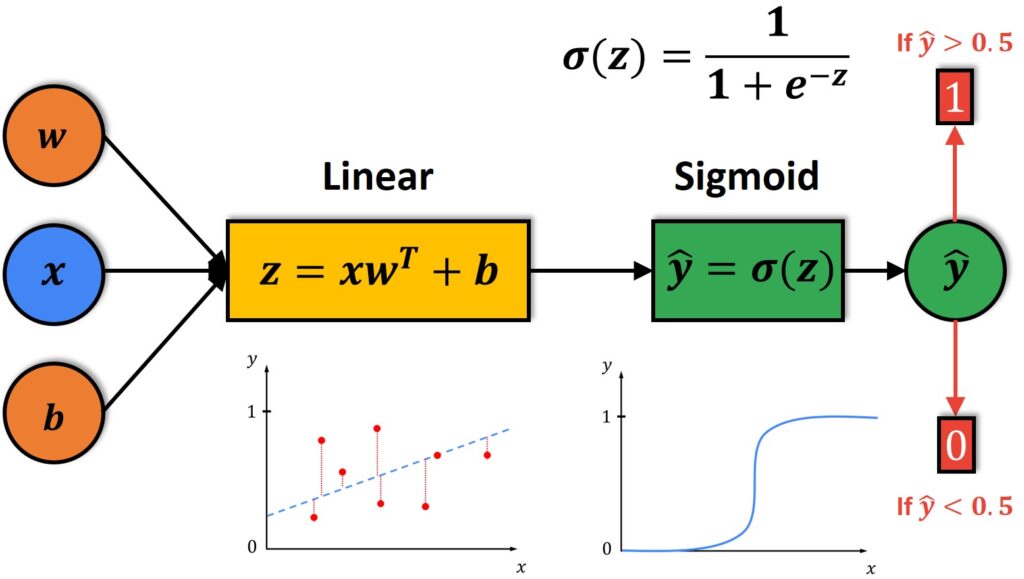
Logistic regression is a statistical model that in its basic form uses a logistic function to model a binary dependent variable, although extensions to the model exist for multiclass classification problems. In contrast to linear regression, which predicts a continuous outcome, logistic regression predicts the probability of an instance belonging to a particular class, making it suitable for classification tasks. The output of a logistic regression model is a value between 0 and 1, which is interpreted as the probability of a given instance being in the ‘positive’ class, labeled ‘1’. The model coefficients are estimated from the training data, usually using a maximum likelihood estimation method, which involves finding the set of coefficients that is most likely to produce the observed set of responses in the training data. This methodology allows for the prediction of class memberships using predictor features, and the coefficients indicate the importance and relationship of each feature to the log odds of the dependent variable. Logistic regression model could be described in the following equations referring to Wikipedia by modeling the parameters in the equations:
p(x)=\frac{1}{1+e^{-(x-\mu) / s}}p(x)=\frac{1}{1+e^{-\left(\beta_{0}+\beta_{1} x\right)}}The following image provides a good illustration for logistic regression, it would be easier for you to learn and understand neural network.
This page contains the detailed description of logistic regression model from scikit-learn. scikit-learn also provides an example for logistic regression for classification of Iris dataset6. A copy of the code will be provided in Canvas with the name “plot_iris_logistic.py”, it can also be download directly here. The source code is provided as follows:
# Code source: Gaël Varoquaux
# Modified for documentation by Jaques Grobler
# License: BSD 3 clause

import matplotlib.pyplot as plt

from sklearn import datasets
from sklearn.inspection import DecisionBoundaryDisplay
from sklearn.linear_model import LogisticRegression

# import some data to play with
iris = datasets.load_iris()
X = iris.data[:, :2]  # we only take the first two features.
Y = iris.target

# Create an instance of Logistic Regression Classifier and fit the data.
logreg = LogisticRegression(C=1e5)
logreg.fit(X, Y)

_, ax = plt.subplots(figsize=(4, 3))
DecisionBoundaryDisplay.from_estimator(
    logreg,
    X,
    cmap=plt.cm.Paired,
    ax=ax,
    response_method="predict",
    plot_method="pcolormesh",
    shading="auto",
    xlabel="Sepal length",
    ylabel="Sepal width",
    eps=0.5,
)

# Plot also the training points
plt.scatter(X[:, 0], X[:, 1], c=Y, edgecolors="k", cmap=plt.cm.Paired)
plt.xticks()
plt.yticks()
plt.show()
In the source code, it is clear to see that the Iris dataset and Logistic Regression Model are imported. You could see that only the first two features are used for the classification purpose, which are sepal length and witdth. After fitting the data to the model, the output figure is presented. The output figure is shown based on these two features as X and Y axis. In the figure, it is aiming to show the decision boundary based on the LogisticRegression model. As you can see the decision boundary is not perfect as there are overlapping of the samples for the classification, this is perhaps because only 2 of the features are used, if we use all the features, it is hard to illustrate in a graph, this example works as a way to illustrate how the logistic regression works.
Random Forest
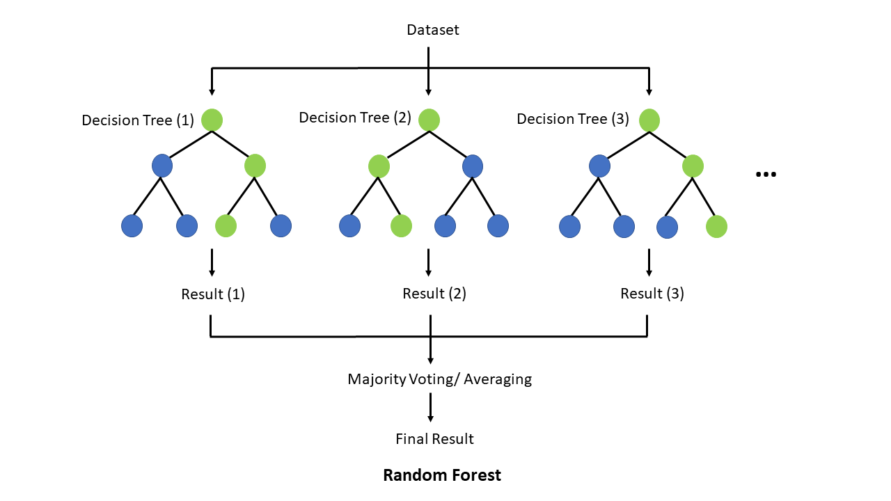
The Random Forest algorithm is an ensemble learning method primarily used for classification and regression tasks that operates by constructing multiple decision trees during training and outputting the class that is the mode of the classes (classification) or mean prediction (regression) of the individual trees. Random forests correct for decision trees’ habit of overfitting to their training set by combining the predictions of numerous trees, each of which is constructed using a random subset of features and samples from the training data. This randomness injects diversity into the model, which, in turn, generally results in a more robust, flexible, and accurate predictive model. Random Forests also provide important insights into feature importance, which can be invaluable in understanding the factors driving the model’s predictions. Scikit-learn page contains the detail about the random forest model.
Here’s an illustration on how random forest works for you to understand.
One special character about random forest is that the decision trees can be shown visually, the following code block is based on this article7.
from sklearn.datasets import load_iris
iris = load_iris()

# Model (can also use single decision tree)
from sklearn.ensemble import RandomForestClassifier
model = RandomForestClassifier(n_estimators=10)

# Train
model.fit(iris.data, iris.target)
# Extract single tree
estimator = model.estimators_[5]

from sklearn.tree import export_graphviz
# Export as dot file
export_graphviz(estimator, out_file='tree.dot',
                feature_names = iris.feature_names,
                class_names = iris.target_names,
                rounded = True, proportion = False,
                precision = 2, filled = True)

# Convert to png using system command (requires Graphviz)
from subprocess import call
call(['dot', '-Tpng', 'tree.dot', '-o', 'tree.png', '-Gdpi=600'])

# Display in jupyter notebook
from IPython.display import Image
Image(filename = 'tree.png')
A decision tree chosen is shown as follows, some terms like gini index are explained here8.
The following code snippet contains the training and testing workflow for random forest from scikit-learn. The script is trying to achieve the classification goal by using all the features.
# Step 1: Import required libraries
from sklearn.datasets import load_iris
from sklearn.ensemble import RandomForestClassifier
from sklearn.model_selection import train_test_split
from sklearn.metrics import classification_report, confusion_matrix, accuracy_score

# Step 2: Load the Iris dataset
iris = load_iris()
X = iris.data
y = iris.target

# Step 3: Split the dataset into a training set and a test set
X_train, X_test, y_train, y_test = train_test_split(X, y, test_size=0.3, random_state=42)  # 70% training and 30% testing

# Step 4: Create a Random Forest Classifier
clf = RandomForestClassifier(n_estimators=100, random_state=42)  # Using 100 trees in the forest

# Step 5: Train the Random Forest Classifier
clf.fit(X_train, y_train)

# Step 6: Predict the response for the test dataset
y_pred = clf.predict(X_test)

# Step 7: Evaluate the model's performance
print("Confusion Matrix:")
print(confusion_matrix(y_test, y_pred))
print("\nClassification Report:")
print(classification_report(y_test, y_pred))
print("Accuracy Score:", accuracy_score(y_test, y_pred))

# Optional: Get feature importances
importances = clf.feature_importances_
print("Feature importances:", importances)

# Optional: Visualize the feature importances
import matplotlib.pyplot as plt

features = iris.feature_names
indices = range(len(importances))
plt.figure(1)
plt.title('Feature Importances')
plt.bar(indices, importances, color='green', align='center')
plt.xticks(indices, features, rotation=90)
plt.tight_layout()
plt.show()
The metrics are given given as results to measure how well the model performs, where the column “support” represents the number of samples that were present in each class of the test set. Sci-kit learn provides the definition of the classification report API9.The more detailed explanation on sci-kit learn’s classification report can be accessed here10.
Confusion Matrix:
[[19  0  0]
 [ 0 13  0]
 [ 0  0 13]]

Classification Report:
              precision    recall  f1-score   support

           0       1.00      1.00      1.00        19
           1       1.00      1.00      1.00        13
           2       1.00      1.00      1.00        13

    accuracy                           1.00        45
   macro avg       1.00      1.00      1.00        45
weighted avg       1.00      1.00      1.00        45

Accuracy Score: 1.0
Feature importances: [0.10410501 0.04460499 0.41730813 0.43398187]
As you can see, the confusion matrix is given, along with the accuracy score and feature importance based on the classification. A confusion matrix is a tabular visualization of the performance of algorithms in machine learning classification tasks, where the actual values of the test data are known. By providing a detailed breakdown of correct and incorrect predictions for each class, the confusion matrix serves as a foundational tool for further metrics such as accuracy, precision, recall, and F1-score, which give deeper insights into the model’s performance, especially in datasets with an uneven class distribution or when certain misclassifications are more significant than others.
Random forest can be tuned based on the following aspects from the article11:
N_estimators: number of tress in random forest.max_depth: maximum depth of each tree in the forest.min_samples_split: minimum number of samples required to split an internal node.min_samples_leaf: minimum number of samples required to be at a leaf node.max_feature: number of features to consider when looking for the best split.
Neural Network
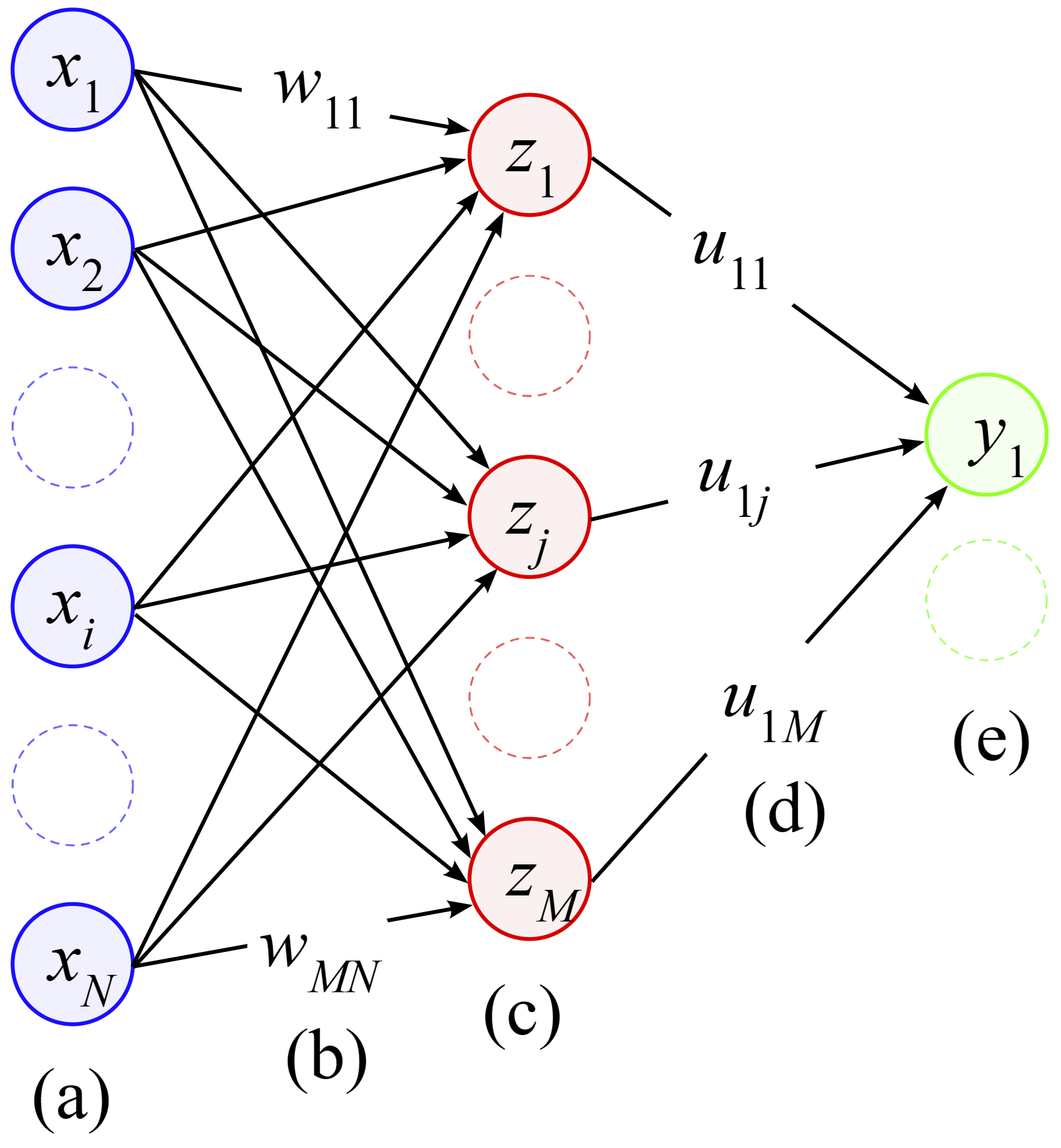
Neural networks consist of layers of interconnected nodes or “neurons,” with each layer responsible for generating increasingly abstract representations of the input data. In a classification context, neural networks take input features and process them through hidden layers using weighted connections and non-linear activation functions, culminating in an output layer that represents the class labels. The network’s weights are adjusted via learning algorithms — typically backpropagation coupled with gradient descent — to minimize the difference between the predicted and actual class labels across multiple instances in the training data. This adaptability makes neural networks particularly suitable for tasks where the relationships between variables are nonlinear and intricate, allowing them to excel in areas ranging from image and speech recognition to medical diagnosis and beyond. Their deep learning variants, which contain many hidden layers, have pushed the boundaries of what’s achievable in classification tasks, setting new benchmarks across various domains.
A neural network can be illustrated as a series of layers, each of which is a function that transforms its input. The input to the first layer is the data, and subsequent layers transform the output of previous layers. The final layer produces the output of the network. The network is trained by adjusting the parameters of the functions so that the output of the network is close to the desired output. This article12 contains useful explanation about multilayer perceptron which is highly recommended for you to understand not only neural network, the history behind the algorithm is also shown. The following image is an illustration of neural network with 1 hidden layer13.
This page in scikit-learn provides the introduction of neural network, various aspects of the algorithm is presented including mathematic formulation, tips and practical uses so that you can have a better understanding of the algorithm. The model for classification is illustrated as follows based on multi-layer perceptron in scikit-learn library.
# Step 1: Import required libraries
from sklearn.datasets import load_iris
from sklearn.neural_network import MLPClassifier
from sklearn.model_selection import train_test_split
from sklearn.preprocessing import StandardScaler
from sklearn.metrics import classification_report, confusion_matrix

# Step 2: Load the Iris dataset
iris = load_iris()
X = iris.data
y = iris.target

# Step 3: Split the dataset into a training set and a test set
X_train, X_test, y_train, y_test = train_test_split(X, y, test_size=0.2, random_state=1)

# Step 4: Data Preprocessing
# It's a good practice to scale the data for neural network convergence
scaler = StandardScaler()
# Compute the mean and standard deviation based on the training data
scaler.fit(X_train)
# Apply the transformations to the data:
X_train = scaler.transform(X_train)
X_test = scaler.transform(X_test)

# Step 5: Create a Neural Network Classifier
# This defines a MLP neural network with two hidden layers, each with 5 nodes.
mlp = MLPClassifier(hidden_layer_sizes=(5, 5), max_iter=1000, random_state=1)

# Step 6: Train the Neural Network
mlp.fit(X_train, y_train)

# Step 7: Predictions and Evaluation
y_pred = mlp.predict(X_test)

# Confusion matrix and classification report
print(confusion_matrix(y_test, y_pred))
print(classification_report(y_test, y_pred))

# Print out the MLP structure
print(mlp)

# You can also explore individual components, like weights and biases.
print("Weights between input and first hidden layer:")
print(mlp.coefs_[0])
print("\nBiases in the first hidden layer:")
print(mlp.intercepts_[0])
In the preceding code, 2 hidden layers with 2 neuron nodes are given for the Iris dataset classification. In addition to the results of the neural network performance, the specific detail on one of the hidden layers is also given.
              precision    recall  f1-score   support

           0       1.00      1.00      1.00        11
           1       1.00      0.92      0.96        13
           2       0.86      1.00      0.92         6

    accuracy                           0.97        30
   macro avg       0.95      0.97      0.96        30
weighted avg       0.97      0.97      0.97        30

MLPClassifier(hidden_layer_sizes=(5, 5), max_iter=1000, random_state=1)
Weights between input and first hidden layer:
[[ 0.59633012  0.43058585 -0.971544   -0.57118375 -0.16776799]
 [-0.58817832 -1.01063668 -0.58940879  0.00651369  0.01601339]
 [-0.70104606  1.18400963 -0.31255475 -0.0423488  -1.24572204]
 [-0.66442217  0.68248851 -0.6290773  -1.33046419 -1.14100224]]

Biases in the first hidden layer:
[1.21996443 1.27916518 0.31004894 0.20325356 1.03175511]
Before the end of the section, here’s a summary14 of different kinds of neural networks.
Misc
Transfer model parameters
I was advised for a situation where you want to save or transfer your trained model, it is actually a good and practical situation. In this case, you can use the library joblib to save your model parameters. Here’s a code snippet for demonstration.
import numpy as np
from sklearn.datasets import load_iris
from sklearn.neural_network import MLPClassifier
from sklearn.model_selection import train_test_split
from sklearn.metrics import accuracy_score
import joblib

# Load the Iris dataset
iris = load_iris()
X, y = iris.data, iris.target

# Split the dataset into training and testing sets
X_train, X_test, y_train, y_test = train_test_split(X, y, test_size=0.2, random_state=42)

# Create and train a scikit-learn MLP neural network model
model = MLPClassifier(hidden_layer_sizes=(10, 5), max_iter=1000, random_state=42)
model.fit(X_train, y_train)

# Make predictions on the test set
y_pred = model.predict(X_test)

# Calculate accuracy
accuracy = accuracy_score(y_test, y_pred)
print(f"Accuracy: {accuracy:.2f}")

# Save the trained model using joblib
model_filename = "iris_neural_network_model.joblib"
joblib.dump(model, model_filename)
print(f"Model saved as {model_filename}")
As you can see, by calling joblib.dump() function, it is easy to store the trained models and reused that in the future.
Extra
Based on what we have learnt on the class, can we apply those knowledge to the news at the moment? For example the dramatic events going on in OpenAI.
- Ilya Sutskever15: Imagenet classification with deep convolutional neural networks16
- Transformer: Attention is All You Need17
- Stable Diffusion: High-Resolution Image Synthesis with Latent Diffusion Models18
- Q*: Everyone’s talking about OpenAI’s Q*. Here’s what you need to know about the mysterious project, OpenAI researchers warned board of AI breakthrough ahead of CEO ouster, sources say.
Conclusion
In this article, the machine learning module scikit-learn is introduced. In addition, 5 types of algorithms based on the module namely: Naïve Bayes, Linear Regression, Logistic Regression, Random Forest and Neural Network are also listed with python detailed code. Thus, by understanding the reason behind each algorithm, you could apply the algorithms on different types of datasets to train machine learning models easily.
Acknolwdgement
Special thanks to Dr. Abhijit Sarkar on his suggestions and feedback for the composition of this post.

- no longer available for students not in 23 Fall Semester[↩]
- Fisher, Ronald A. “The use of multiple measurements in taxonomic problems.” Annals of Eugenics 7, no. 2 (1936): 179-188.[↩]
- refer from the site https://www.biosymetrics.com/blog/binary-classification-metrics[↩]
- https://yury-zablotski.netlify.app/post/confusion-matrix/[↩]
- Sandipan Dey, “Probabilistic Deep Learning with Tensorflow”, 2021[↩]
- This is example is recommended by Professor Sarkar[↩]
- Koehrsen, Will, “How to Visualize a Decision Tree from a Random Forest in Python using Scikit-Learn”, 2018.[↩]
- Dash, Shailey, “Decision Trees Explained — Entropy, Information Gain, Gini Index, CCP Pruning”, 2022[↩]
- sklearn.metrics.classification_report[↩]
- Amir Masoud Sefidian, Understanding Micro, Macro, and Weighted Averages for Scikit-Learn metrics in multi-class classification with example[↩]
- Ben Fraj, Mohtadi, “In Depth: Parameter tuning for Random Forest”, 2017[↩]
- The Multilayer Perceptron – Theory and Implementation of the Backpropagation Algorithm[↩]
- INKSCAPE, Artificial Neural Network N-M-1[↩]
- Fjodor van Veen, Asimov Institute, “The Neural Network Zoo”, 2019. 📷[↩]
- Ilya Sutskever Google Scholar[↩]
- Krizhevsky, Alex, Ilya Sutskever, and Geoffrey E. Hinton. “ImageNet classification with deep convolutional neural networks.” In Advances in neural information processing systems, 25:1097-1105. 2012.[↩]
- Vaswani, Ashish, Noam Shazeer, Niki Parmar, Jakob Uszkoreit, Llion Jones, Aidan N. Gomez, Łukasz Kaiser, and Illia Polosukhin. “Attention is all you need.” In Advances in neural information processing systems, 30:5998-6008. 2017.[↩]
- Rombach R, Blattmann A, Lorenz D, et al. “High-resolution image synthesis with latent diffusion models”. Proceedings of the IEEE/CVF conference on computer vision and pattern recognition. 2022: 10684-10695.[↩]
Leave a Reply