Part of the Train a Transformer on Silicon series — start at #0.
Building a transformer that trains itself in hardware — from a numpy model down to a chip layout. This is the intro; the details (and the pretty pictures) come in the posts that follow.
Why training, not inference
Most “AI chips” are inference accelerators — they run a model that was already trained somewhere else, usually on a rack of GPUs. That’s the easy 90%.
I wanted to build the hard 10%: a chip that does the training itself — the backward pass, the gradients, the weight updates. So the plan for this series is simple to state:
Build a digital chip that trains a transformer on-chip — forward pass, backpropagation, and the weight update, all in hardware — and take it through the full flow to an actual layout.
No GPU in the loop. The silicon does the learning.
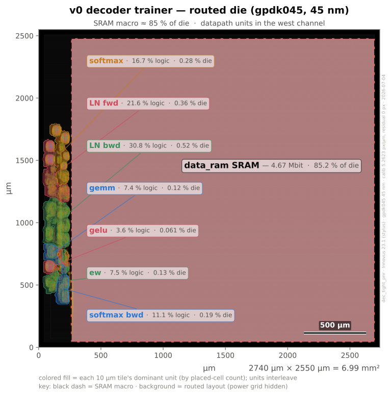
This is where the series ends up — a 6.99 mm² layout on a generic educational 45 nm PDK (gpdk045) that trains a small transformer decoder; ~85 % of it is one SRAM macro, all the compute is the thin channel on the west edge. The next posts break it down; the figure-making pipeline has its own post.
This first post is just the setup: what I’m building, how I’m going to convince myself it works, and what’s coming. I’ll add the numbers, waveforms, and layout images as the series goes — and I’ll be honest about the limitations the whole way.
What “training on a chip” involves
A single transformer layer is manageable on paper: normalization, self-attention with a softmax, a feed-forward network, and residual connections. Training makes it more interesting, because the hardware now also has to:
- run the forward pass and remember the intermediate values,
- run the backward pass — push gradients back through the softmax, the norm, the activation, and a stack of transposed matrix multiplies, and
- update the weights in place.
My approach is a shared datapath: one matrix-multiply engine plus a few small units for the nonlinearities, time-multiplexed across the whole forward/backward/update loop by a little on-chip controller. It’s not the fastest way to do it — but it’s small, and it scales nicely (bigger models mostly cost more memory and more cycles, not more logic). Everything runs in fixed-point (Q16.16), no floating point.
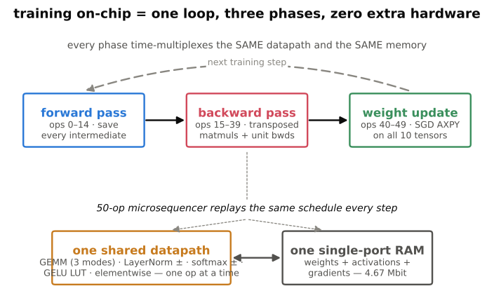
The loop the silicon runs: forward pass leaves a trail of intermediates, the backward pass reads them to make gradients, and the update folds those gradients back into the weights — then it does it again.
What the silicon actually computes
“A layer plus its backward pass” is easy to say and easy to hand-wave. Here’s the honest, stage-by-stage list of what the hardware has to do — forward first, then backward. Everything reduces to a handful of primitives: multiply-accumulate (MAC), add/subtract/multiply, compares, shifts, and a small set of lookup tables.
| stage | forward | backward |
|---|---|---|
| LayerNorm | per-row mean (sum + shift), variance (sum of squares + shift), 1/\sqrt{\sigma^2+\epsilon} via LUT, normalize multiplies, learnable \gamma/\beta multiply-add | the mean/variance coupling terms — per-row sums of d\hat{x} and d\hat{x}\cdot\hat{x} — plus \gamma and \beta gradients (reductions across rows) |
| Q/K/V + all matmuls | MAC (A\cdot B) | MAC, but transposed: A^{\mathsf{T}}B for weight gradients, AB^{\mathsf{T}} for input gradients — same multiplies, different address order |
| Attention scores | MAC (QK^{\mathsf{T}}) + a constant scale multiply (1/\sqrt{d}) | flows through the softmax and matmul backwards |
| Causal softmax | per-row max (compares), subtract, exp via LUT, sum (accumulate), reciprocal via LUT, normalize multiplies; masked positions zeroed | dS = A\cdot\big(dA \,{-}\, \mathrm{rowsum}(A\cdot dA)\big) — multiplies plus a per-row reduction |
| GELU | one LUT returning both \mathrm{gelu}(x) and \mathrm{gelu}'(x) | just an elementwise multiply with the saved derivative |
| Residual adds | elementwise add | gradient flows straight through |
| MSE loss | — | elementwise subtract + constant scale (2/N) |
| SGD update | — | AXPY: W \leftarrow W \,{-}\, \mathrm{lr}\cdot\mathrm{grad}, applied to all 10 parameter tensors (\gamma/\beta included) |
The thing worth noticing: backprop introduces no new arithmetic. It’s the same MACs the forward pass runs, mostly in their transposed form, plus a few per-row reductions. The GEMM engine is one block with three modes — A\cdot B, A^{\mathsf{T}}B, AB^{\mathsf{T}} — and those three cover every matrix multiply in both directions.
Attention, concretely
It’s worth assembling those table rows into the actual attention computation once, because the hardware view of it is unusual. On paper, one head of causal self-attention over the normalized input y_1 is:
Q = y_1 W_q, \qquad K = y_1 W_k, \qquad V = y_1 W_v
S = \frac{QK^{\mathsf{T}}}{\sqrt{d}}, \qquad A_{ij} = \frac{e^{\,S_{ij}-m_i}}{\sum_{k \le i} e^{\,S_{ik}-m_i}} \;\; (j \le i), \qquad \mathrm{attn}(y_1) = (A\,V)\,W_o
where m_i = \max_{k \le i} S_{ik} is the per-row max (subtracted for numerical range — it’s also what keeps the exp LUT’s argument \le 0), and the j \le i condition is the causal mask: position i may only attend to itself and earlier positions.
In the hardware, there is no attention unit. That whole expression is a schedule — eight consecutive ops of the sequencer’s program, run one at a time through the same two blocks:
- ops 1–3: three GEMMs — Q, K, V projections
- op 4: one GEMM in transpose mode — S = QK^{\mathsf{T}} (the
tbflag again; no transpose hardware) - op 5: one elementwise SCALE — multiply by 1/\sqrt{d}, which for d = 64 is exactly 1/8
- op 6: the causal softmax — per row: max, subtract, exp LUT, accumulate, reciprocal LUT, normalize
- ops 7–8: two more GEMMs — \mathrm{ctx} = A\,V, then the output projection \mathrm{ctx}\,W_o
So “computing attention” costs six matrix multiplies, one scale, and one softmax pass — and the backward pass reuses the same schedule shape with the transposed GEMM modes plus the softmax backward (dS = A\cdot(dA \,{-}\, \mathrm{rowsum}(A\cdot dA)), one more FSM). The exotic-sounding part of a transformer turns out to be the most conventional part of the chip: it’s almost entirely the GEMM engine, called seven times with different base addresses.
The loss, and why it’s MSE (not cross-entropy — yet)
Every training step needs a number to descend on. v0 uses plain mean-squared error over the layer’s output:
L = \frac{1}{N}\sum_{t,j}\big(X^{\mathrm{out}}_{tj} \,{-}\, T_{tj}\big)^2, \qquad \frac{\partial L}{\partial X^{\mathrm{out}}} = \frac{2}{N}\big(X^{\mathrm{out}} \,{-}\, T\big)
with N = T\cdot D = 1024, and the target T is just the input sequence shifted by one position — a causal copy task: “predict the next vector.” It has no vocabulary and no meaning, but it forces the causal attention to do its job, and that’s all v0 needs to prove.
The honest answer to “why not cross-entropy” is that v0 has nothing to be cross-entropic about. Cross-entropy is the right loss when the model emits a probability distribution over discrete tokens — which requires an embedding table on the way in, an unembedding projection (D \to V logits) on the way out, and a softmax over the vocabulary. None of that hardware exists yet; it arrives together with the vocabulary in a later post. When it does, cross-entropy comes almost for free: its gradient through the softmax is the famously clean p \,{-}\, y, and the softmax machinery is already on the die. Until then, bolting a token loss onto a model with no tokens would be theater.
MSE, meanwhile, is nearly free in silicon. Its gradient is one elementwise pass — subtract, then scale by 2/N — which is exactly opcode 5 of the elementwise unit (SUBSC: C=(A-B)*k). And because N = 1024 is a power of two, 2/N = 2^{-9} is exact in Q16.16 — no rounding in the one constant that seeds the entire backward pass. That output gradient \partial L/\partial X^{\mathrm{out}} is where backprop starts; everything in ops 16–39 exists to carry it backward.
SGD: the whole optimizer is one instruction
Once the backward pass has left every gradient sitting in RAM, the update is:
W \leftarrow W \,{-}\, \eta\,\frac{\partial L}{\partial W}, \qquad \eta = 2^{-5} = 0.03125
applied tensor by tensor — ops 40–49 of the schedule, one AXPY pass each over W_q, W_k, W_v, W_o, W_1, W_2 and the four LayerNorm parameters \gamma_1, \beta_1, \gamma_2, \beta_2. The learning rate is a power of two on purpose: \eta\cdot\mathrm{grad} in fixed point is then exact, not approximated. The update happens in place — each weight is read, adjusted, and written back to the same address it has always lived at. Nothing is copied anywhere; the chip quietly rewrites itself.
Why plain SGD, when everything serious trains with momentum or Adam? Memory. Momentum keeps one extra state tensor per weight (2× weight-adjacent memory); Adam keeps two (3×). On a chip, optimizer state isn’t a hyperparameter — it’s silicon area, and memory already dominates this die. Vanilla SGD keeps zero extra state: the weights are the entire training state of the machine. It converges slower and noisier, and that’s a trade I’ll measure properly when a fancier optimizer gets its own post. For proving the mechanism, SGD is the honest minimum.
The LUT inventory
There is no divider, no square-root unit, and no exponential unit anywhere in the design. Every transcendental is a table. Four of them replace all the “hard” math:
rsqrt_lut— 1/\sqrt{x}, 1024 entries + linear interpolation. Used by LayerNorm (and by RMSNorm in the earlier encoder baseline).exp_lut— e^{x} for x \le 0, 1024 entries + interpolation. Inputs are pre-shifted by the row max, so the argument is always \le 0. Used by softmax forward.recip_lut— 1/x, 1024 entries + interpolation. Used by softmax normalization — and anywhere else a divide would appear, because there are none.- the GELU LUT — 512 entries over [-4, 4), piecewise-constant (no interpolation), returning the pair \big(\mathrm{gelu}(x),\, \mathrm{gelu}'(x)\big); outside the range it clamps to the identity/zero asymptotes.
Table-plus-interpolation is a deliberate area/accuracy trade — cheaper than a real function unit, close enough in Q16.16. It also has quirks: the exp table returns \exp(0) = 0.9845, not exactly 1.0. I don’t fix that. The numpy golden model parses the same tables straight out of the RTL, so both sides share the quirk bit-for-bit — which is the whole point, because the verification story (next section) is bit-exactness, and you can only be bit-exact with the quirks, not against them.
So the full operation census is small: MAC, add/subtract/multiply, compare, shift, and four LUTs. That’s exactly why one shared datapath can serve the entire training loop — the hard part turns out to be sequencing and memory, not exotic arithmetic. More on that when I get to the numbers.
What each block looks like in RTL
That census is small, and so is the hardware. Every unit is built to the same recipe, so once you’ve read one you’ve mostly read them all — and that sameness is a big part of what makes the whole thing tractable. A quick tour.
The shared pattern
Every unit is the same shape: a small finite-state machine that owns no memory of its own. It walks one shared, single-port RAM one address at a time — issue an address, wait a cycle for the data to land, capture it — and does fixed-point math in Q16.16, where a multiply is two Q16.16 numbers producing a Q32.32 product that gets rounded and saturated back with (prod + 2¹⁵) >>> 16. That’s the entire vocabulary. Here it is in the GEMM engine, the one block every matrix multiply runs through:
wire [AW-1:0] addrA = ta ? (baseA + k*M + i) : (baseA + i*K + k);
wire [AW-1:0] addrB = tb ? (baseB + j*K + k) : (baseB + k*N + j);
// …
S_RDA:  begin mem_addr<=addrA; st<=S_LATA; end          // issue A read
S_LATA: begin mem_addr<=addrB; st<=S_RDB;  end          // A on bus next cyc; issue B read
S_RDB:  begin a_val<=mem_rdata; st<=S_LATB; end         // capture A
S_LATB: st<=S_MAC;                                      // B on bus next cyc
S_MAC:  begin
          acc <= acc + ($signed(a_val) * $signed(mem_rdata)); // capture B & MAC
          if (k == K-1) st<=S_WR; else begin k<=k+1; st<=S_RDA; end
endThe interesting lines are the two addr ternaries. ta and tb are the whole story of backprop matmuls: forward is A\cdot B, the weight gradient needs A^{\mathsf{T}}B, the input gradient needs AB^{\mathsf{T}}. Transposing a matrix here is not new hardware — it’s reindexing the same reads (k*M + i instead of i*K + k). Same multipliers, same accumulator, different address arithmetic. One engine, all three modes, forward and backward.
Lookup tables instead of function units
Each transcendental is a table with linear interpolation. exp_lut is representative:
module exp_lut(input signed [31:0] x, output reg signed [31:0] y);
    wire signed [31:0] si = x >>> 10;
    wire [10:0] idx  = lo?11'd0 : hiz?11'd1023 : (si[10:0]+11'd1024);
    wire [9:0]  frac = x[9:0];
    // … case(idx) → y0, case(idxp) → y1 : the two neighbouring table entries …
y = y0 + ((($signed(y1)-$signed(y0))*$signed({1'b0,frac})) >>> 10);si = x >>> 10 picks one of 1024 segments, two case statements fetch that segment’s endpoints y0/y1, and the last line linearly interpolates between them using the low bits as frac. That’s how exp, reciprocal, and rsqrt all exist without a single divider, exp, or sqrt unit on the die.
GELU takes it further — its table returns two values at once:
module gelu_unit(input signed [31:0] x, output reg signed [31:0] y, output reg signed [31:0] dy);
    // … 512-entry case over [−4,4) sets g (= gelu) and d (= gelu′) …
    if (hi)      begin y=x;     dy=32'h00010000; end
    else if (lo) begin y=32'h0; dy=32'h0;        end
else begin y=g; dy=d; end512 entries, piecewise-constant, returning both \mathrm{gelu}(x) and \mathrm{gelu}'(x); the hi/lo branches clamp to the identity/zero asymptotes outside the range. Because the derivative is looked up alongside the value, GELU’s backward pass is a single multiply against the saved dy.
Multi-pass units carry state through memory
LayerNorm can’t be done in one sweep — it needs the mean before it can compute the variance — so it’s three passes over each row, and the FSM’s state list reads like the math:
localparam IDLE=0, P1_RD=1,P1_LAT=2,P1_ACC=3, MU=4,
           P2_RD=5,P2_LAT=6,P2_ACC=7, VAR=8, RSQ=9, WRR=10,
           P3_RD=11,P3_LAT=12,P3_XH=13, P3_RG=14,P3_LG=15,P3_GM=16,
           P3_RB=17,P3_LB=18,P3_WY=19, DONE=20;
// …
MU:     begin mu <= sat(acc >>> LOG2D); acc<=0; st<=P2_RD; end
// …
WRR: begin mem_we<=1; mem_addr<=baseR+row; mem_wdata<=r_reg; st<=P3_RD; endPass 1 sums x and divides by D — and because D is a power of two, “divide by D” is >>> LOG2D, a shift. Pass 2 sums the squared deviations; RSQ hits the rsqrt table; pass 3 writes xhat and y. Look at WRR: it writes r (and later xhat) back to RAM for the backward pass to read. That is where training’s memory cost first shows up in the RTL — the forward pass has to leave a trail behind it.
Causality is a loop bound
The entire difference between a decoder and an encoder — the thing the next post is named after — is one comparison in the softmax FSM:
M_ACC: begin
         if($signed(mem_rdata)>$signed(maxv)) maxv<=mem_rdata;
         if(k==row) begin k<=0; sum<=0; st<=E_RD; end     // causal: stop at diagonal
         else begin k<=k+1; st<=M_RD; end
endRow i scans columns 0..i and stops. if(k==row) is the causal mask — no masking logic, no -\infty additions; the loop just ends at the diagonal, and a later pass zero-fills the columns to the right.
The optimizer is an opcode
The elementwise unit is a five-mode mini-ALU, and SGD is just one of its modes:
//   0 ADD   C=A+B        1 SUB   C=A-B       2 MUL  C=A*B (fixed)
//   3 SCALE C=k*A        4 AXPY  C=A-k*B (SGD: A=W, B=grad, k=lr)
//   5 SUBSC C=(A-B)*k    (loss grad: (X2-T)*k, k=2/N)
// …
wire signed [2*W-1:0] kB = ($signed(mem_rdata)*$signed(konst)+(1<<<(FRAC-1)))>>>FRAC;
// …
4: res = sat($signed(a_reg)-kB);W \leftarrow W \,{-}\, \mathrm{lr}\cdot\mathrm{grad}, the entire weight update, is op 4 — A \,{-}\, k\cdot B, run across all ten parameter tensors. No optimizer block; an opcode.
The conductor
None of those units knows what it’s part of. The schedule lives in one big case in the top-level trainer — 50 hardcoded ops, each naming a unit, its base addresses, and its dimensions:
0: begin sel=2; aB=51200; aC=51264; aD=51456; aE=52480; aF=53504; m0=16; m1=64; end
1: begin sel=1; aA=51456; aB=2048; aC=53520; m0=16; m1=64; m2=64; end
// …
40: begin sel=5; ewop=4; aA=2048; aB=130336; aC=2048; m0=4096; kk=K_LR; endsel picks the unit (2 = LayerNorm, 1 = GEMM, 5 = elementwise), the a* fields are RAM base addresses, m* are the dimensions. So op 0 is the first LayerNorm, op 1 is the Q projection (y_1 W_q, on the normalized input), and op 40 is W_q \leftarrow W_q \,{-}\, \mathrm{lr}\cdot dW_q. Ops 0–14 are the forward pass, 15–39 the backward pass, 40–49 the SGD updates. The “program” is a fixed timetable, not fetched instructions.
The whole trainer is about seven small FSMs, four tables, and one case statement — no floating point, no divider, no cache, no surprises. That is exactly what makes it verifiable bit-for-bit, which is the next section’s subject.
Why the chip is mostly memory
Look again at the die at the top of this post. The compute — those seven state machines and four tables — is the thin strip on the left. Everything else, roughly five-sixths of the silicon, is one block of SRAM. That ratio isn’t a quirk of this design; it’s what training costs. Here is the entire 4.67 Mbit RAM, sorted by what lives in it:
| what’s in the RAM | words | share | on an inference chip? |
|---|---|---|---|
| model weights | 49,408 | 34 % | yes |
| weight gradients | 49,408 | 34 % | no |
| forward activations, saved for the backward pass | 25,120 | 17 % | no |
| activation gradients + backward scratch | 19,968 | 14 % | no |
| inputs + target | 2,048 | 1 % | inputs only |
| total | 145,952 | 4.67 Mbit |
Only the first row — the model’s own parameters — would exist on a chip that merely ran this network. The other two-thirds is there purely because this chip learns, and it breaks into three costs, each a direct consequence of backpropagation.
Every weight needs a gradient. SGD updates each parameter by W \leftarrow W \,{-}\, \eta\,\partial L/\partial W, so for every weight there is a gradient of exactly the same shape waiting in memory. The gradient block is the same size as the weight block, to the word — 49,408 each. And that is the cheap case: plain SGD keeps nothing else. Momentum would add another full copy of the model; Adam, two more. On a chip, “which optimizer” is really “how many times over do I store the model” — which is why v0 uses the one optimizer that stores it zero extra times.
The forward pass can’t forget. The weight gradient for a matmul is \partial L/\partial W = A^{\mathsf{T}}\,\partial L/\partial \mathrm{out} — it needs the activation A that the weight multiplied on the way forward. So every intermediate the forward pass produces must be kept until the backward pass reads it. Inference computes an activation, uses it, and overwrites it a moment later; training has to leave the whole trail behind — 25,120 words of it here. (Those xhat and r writes in the LayerNorm FSM, a few sections up, were exactly this: the forward pass stashing what backprop will need.)
The backward pass has its own working set. Gradients flow back through the same graph the forward pass ran, and each stage needs scratch for the gradient it hands to the next — dS, d\mathrm{ctx}, dQ, and the rest — another 19,968 words.
Add it up and training this layer needs on the order of three times the memory that running it would. And v0 is the naive version: all 145,952 words are live at once, every buffer parked at a fixed address for the entire run, nothing ever reused. Most of those buffers are dead for most of a step — which is the first thing worth fixing, and a story for a later post.
How I’ll keep myself honest
It’s easy to write hardware that looks like a transformer. It’s hard to prove it actually learns. So the rule for the whole project is check the math first:
- Write the entire thing — forward, backward, weight update — in numpy at the exact precision the hardware will use.
- Check the backpropagation against a known-good autograd implementation. If the gradients don’t match, stop — the hardware can’t fix bad math.
- Only then write the RTL, and make it reproduce those reference numbers.
That “golden-model-first” habit is boring but it’s what makes the results trustworthy — and it’s a big part of what I want to show in this series.
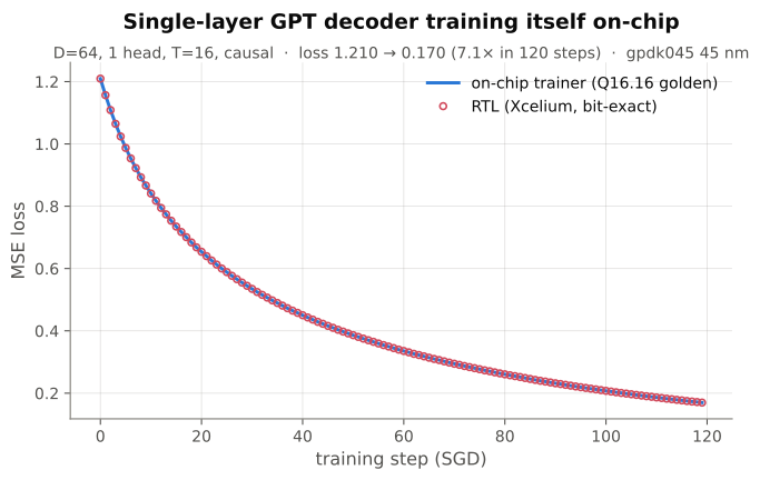
The payoff of golden-model-first — the RTL’s training trajectory (dots) sits exactly on the fixed-point golden model (line), bit-for-bit.
Where things stand
A first version already runs end-to-end — the die at the top of this post is it: a single GPT-style decoder layer that trains on-chip and comes out as a clean layout on a generic 45 nm process. The next posts break down the numbers, the layout, and the bug that fooled me. For now the takeaway is just: the mechanism works — a small block of silicon that, given data, sits there and learns.
Honest caveats (up front)
I only think a project like this is worth writing about if it’s honest about what it is:
- It’s tiny — a demonstration of the mechanism, not a competitive accelerator.
- It’s a generic, educational process, not a real foundry PDK — the numbers are representative, not signoff-grade.
- No tape-out — this is a clean layout in the design tools, not a fabricated chip.
The interesting parts, honestly, are the things that broke along the way — and I’ll tell those stories as they come up. The debugging is where the real learning is.
What’s next
The full roadmap for the series lives in Part 0. Next, I build the minimal version — a GPT-style decoder trainer, which turns out to be “the encoder plus a causal mask.”
If you build hardware, do ML, or work in chip design, follow along — and if you catch something wrong, tell me. That’s the best thing that can happen to a post like this.
Next up: “A decoder is just an encoder with a mask.”
- ($signed(y1)-$signed(y0[↩]
Leave a Reply